Tasks and Pipeline Graphs#
A pipeline is represented as a graphs (PipelineGraph) of tasks
(PipelineTask), where each task, in addition to containing runtime
configuration, references a function that follows the signature:
def task(df: pandas.DataFrame, ...) -> pandas.DataFrame
A graph then connects the outputs of one task to the input of another. For example, consider the graph:
t1 = PipelineTask('task1', task1_func)
t2 = PipelineTask('task2', task2_func)
t3 = PipelineTask('task3', task3_func)
PipelineGraph([(t1, t2), (t1, t3)])
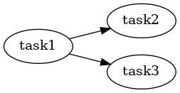
which has a single input and two outputs. As can be seen above, the task graph need not be a simple path (linear where no task has more than a single input/output), though some executors may place restrictions on the geometry.
Task units#
As can be deduced from the signature above, a task does work on a batch of data (which can be 1 or more rows) and
produces a batch of data. The PipelineTask wraps the actual task function
both to provide an abstraction between the business logic (what the pipeline should do) and the coordination (this
framework), and because the design is around scaling of execution on potentially large and heterogeneous compute
infrastructure. As such, it contains settings for things like the number of CPUs or GPUs required to execute a single
batch of data, other arbitrary resources such as the presence of a local database, and the batch size to feed a single
execution of the task.
For example, consider a few possible scenarios of tasks:
A machine learning inference step that requires GPUs, where the loading of the model is expensive and runtime small enough that it is reasonable to amortize the loading cost over several rows:
PipelineTask('do_inference', inference_function, batch_size=20, num_gpus=1)
A multi-core database lookup step with data loading overhead. Runtime of 1000 inputs similar to a single input (colabfold search step behaves this way in certain circumstances sokrypton/ColabFold). Note also the custom resource identifying the database, which is large and stored on local disk due to IO sensitivity - this ensures we run on a host that has the database installed:
PipelineTask('colabfold_mmseqs', colabfold_search, batch_size=1000, num_cpus=32, resources={'colabfold_db': 0.01})
A long-running simulation step. Here we benefit from multiple cores, but we want to decrease the cost of potential failure due to the long runtime - so single row input:
PipelineTask('dft', run_simulation, batch_size=1, num_cpus=16)
Fast task, no particular batching or resource requirements. No re-batching, so input is size of previous task output:
PipelineTask('task', fast_task)
These settings are obviously task dependent, further what is correct in one runtime environment might not be the same as
another, so all these settings can be configured at runtime (see also Executing Pipelines) - so the definition of
PipelineTask can be considered defaults. See Configuring Pipelines for more
details.
Graph construction#
PipelineGraph is a subclass of DiGraph, and
accepts the same edge list formats as that. Generally, this will take the form:
[(PipelineTask, PipelineTask), ...]
e.g. a list of edges directing from task to task. Given that many useful pipelines will be simple path graphs, a graph can also be constructed from a list of tasks, where edges are implicit between all elements, directing from left to right:
[PipelineTask, ...]
There are three kinds of tasks in a graph:
Those that have no input edges.
These are sources. They still consume a DataFrame, but their input data come from the executor and by default represent just a sequence number for the present batch - the task will generally generate relevant data here. See Executing Pipelines for more details on how pipelines are run and data generation.
Those that have no output edges.
These are sinks. The output of these task are yielded to the caller of the pipeline
run()method, and, for example, can be written to disk in parquet (e.g. inwriteto()).Those with both input and output edges.
These tasks consume batches from the task originating at input edges, and feed outputs to those at the terminating end of output edges.
Graph operations#
In addition to any networkx utilities to operate on or analyze the graph, the
PipelineGraph has some methods to identify the
source_tasks (those that have no input edges) and
sink_tasks (those that have no output edges) to walk the graph
in a breadth-first-search, by default from the sources to the sinks, see walk.
Multiple edges#
Here are how multiple edges are processed in a pipeline:
Tasks that have multiple output edges will send a copy of each output batch to each of the nodes at the other end of the edge. This effectively increases the number of output rows sent to following tasks of the pipeline, since, as below, there is no join mechanism. However, subsequent tasks may always perform a filter on batches.
Joining of rows using final output separately is always possible, of course.
Tasks that have multiple input edges will take a batch separately from each of the input tasks and process it in the order queued. The batches input are separate entities, however they are subject to merging per the batch size of the input. For example, for the following pipeline:
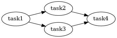
assuming task2 and task3 emit batches of size 10, and task4 consumes batches of size 20, it might occur that the executor combines the rows of one batch of task2 with rows from one batch of task3 and sends that input to task4. Note that there is no mechanism to join (in the relational sense) the rows of task2 to the rows of task1, only union them.